This is a technical breakdown of a research project I built during my fifth semester at Howest. The goal: build an end-to-end machine learning pipeline entirely in Rust using the Burn framework, train a plant disease classifier with minimal labeled data through semi-supervised learning, and deploy it offline across desktop, browser, and mobile.
The implementation, experiment artifacts, and thesis documentation are available in the public repository.
The Problem
Plant disease detection for farmers in areas with limited or zero internet connectivity. Expert labeling and laboratory workflows can be costly and slow, while cloud inference requires a stable connection. Neither assumption is reliable in every field setting.
The requirements:
- Must work 100% offline
- Must run on devices farmers already own (phones, laptops)
- No installation complexity (farmers are not sysadmins)
- Sub-second inference for real-time feedback
On top of that, labeled agricultural data is expensive. Expert annotation runs about €2 per image. For 50,000 images, that is €100K we do not have. So the pipeline needs to learn effectively from a small labeled subset.
Why Rust and Burn
I chose Rust and Burn (v0.20.0-pre) because the constraints of this project play directly to Rust's strengths.
Single-Binary Deployment
Burn compiles to a single binary with no external
runtime dependencies. With LTO and
codegen-units = 1 in the release profile,
the entire model and inference runtime ship as one
file. No virtual environments, no dependency managers,
no installation steps. For farmers who are not going to
run pip install, this matters.
Multi-Backend from One Codebase
Burn supports multiple compute backends through Rust's trait system:
-
burn-cudafor native CUDA (desktop GPU training and inference) -
burn-wgpufor cross-platform GPU via Vulkan, Metal, and DX12 -
burn-ndarrayfor pure-CPU fallback with zero dependencies
The same model definition compiles to all of these. Same weights, different targets, one language from training to production.
Instant Startup
Burn loads in under 100ms. For a mobile app where users expect instant feedback, startup time matters as much as inference time.
Model Architecture
The classifier is a compact CNN with four convolutional blocks, totaling around 460,000 parameters. The architecture:
Input: [B, 3, 128, 128]

Conv2d(3, 32, 3x3, pad=same)   -> BatchNorm -> ReLU -> MaxPool(2x2)
Conv2d(32, 64, 3x3, pad=same)  -> BatchNorm -> ReLU -> MaxPool(2x2)
Conv2d(64, 128, 3x3, pad=same) -> BatchNorm -> ReLU -> MaxPool(2x2)
Conv2d(128, 256, 3x3, pad=same)-> BatchNorm -> ReLU -> MaxPool(2x2)

AdaptiveAvgPool2d(1x1) -> Flatten
Linear(256, 256) -> ReLU -> Dropout(0.3)
Linear(256, 38)

Output: [B, 38] logits
Input images are 128x128 RGB, normalized with ImageNet statistics (mean = [0.485, 0.456, 0.406], std = [0.229, 0.224, 0.225]). The output covers 38 plant disease classes from the PlantVillage dataset.
The Burn model definition makes the backend generic
through the B: Backend trait bound. This
exact struct compiles to CUDA, CPU, or wgpu with no
code duplication:
#[derive(Module, Debug)]
pub struct PlantClassifier<B: Backend> {
    conv1: Conv2d<B>,
    bn1: BatchNorm<B, 2>,
    conv2: Conv2d<B>,
    bn2: BatchNorm<B, 2>,
    conv3: Conv2d<B>,
    bn3: BatchNorm<B, 2>,
    conv4: Conv2d<B>,
    bn4: BatchNorm<B, 2>,
    fc1: Linear<B>,
    fc2: Linear<B>,
}
Semi-Supervised Learning Pipeline
This is the core of the project. With only 20% of the data labeled, I needed a way to leverage the remaining 80%. The approach: iterative pseudo-labeling (also called self-training).
Data Splitting
The ~87,000 PlantVillage images are split in a stratified manner:
Total dataset (~87K images)
  |-- Test set:       10% (~8.7K)   -- never seen during training
  |-- Validation set: 10% (~8.7K)   -- for monitoring and early stopping
  |-- Remaining:      80% (~69.6K)
       |-- Labeled pool:  20% (~13.9K)  -- used for supervised training
       |-- Stream pool:   80% (~55.7K)  -- unlabeled, used for SSL
The Pseudo-Labeling Algorithm
The idea is simple: train a model on what you have, use it to label what you do not, then retrain on the expanded dataset. But the details determine whether this works or spirals into noise.
For each unlabeled sample $x_u$, the model produces:
$$p = \text{softmax}(f(x_u))$$The predicted class and confidence score are:
$$\hat{y} = \arg\max(p), \quad c = \max(p)$$A pseudo-label is accepted only when the confidence exceeds a threshold $\tau$:
$$c \geq \tau \quad (\tau = 0.9)$$This 90% threshold is strict by design. Accepting low-confidence predictions poisons the training set. The final evaluation did not independently recompute pseudo-label precision, so the threshold is treated as a pipeline control rather than a reported result.
Loss Function
For labeled data, the loss is standard cross-entropy:
$$\mathcal{L}_{\text{labeled}} = -\frac{1}{N}\sum_{i=1}^{N} \log\left(\text{softmax}(f(x_i))_{y_i}\right)$$For pseudo-labeled data, a confidence-weighted negative log-likelihood is used. Each sample's contribution is scaled by how confident the model was when it generated the pseudo-label:
$$\mathcal{L}_{\text{pseudo}} = \frac{\sum_{i=1}^{M} w_i \cdot \left(-\log\left(\text{softmax}(f(x_i))_{\hat{y}_i}\right)\right)}{\sum_{i=1}^{M} w_i + \epsilon}$$where $w_i$ is the confidence score of pseudo-label $i$ and $\epsilon = 10^{-8}$ prevents division by zero.
The total loss combines both with a ramp-up schedule:
$$\mathcal{L}_{\text{total}} = \mathcal{L}_{\text{labeled}} + \lambda \cdot \text{ramp}(t) \cdot \mathcal{L}_{\text{pseudo}}$$The ramp-up function linearly increases the pseudo-label weight over the first $T_{\text{ramp}}$ epochs:
$$\text{ramp}(t) = \min\left(\frac{t}{T_{\text{ramp}}}, 1\right), \quad T_{\text{ramp}} = 10$$This prevents the model from being overwhelmed by pseudo-labels early in training, when the predictions are still unreliable.
The Simulation Loop
The SSL pipeline simulates a realistic deployment scenario where new images arrive daily (like a farmer photographing crops over time):
- Supervised pre-training on the 20% labeled pool using cross-entropy with Adam (lr = 0.0001, weight decay = 1e-4).
- Daily inference on batches of 100 images from the stream pool.
- Confidence filtering at $\tau = 0.9$, with a per-class cap of 500 pseudo-labels to prevent class imbalance.
- Buffer accumulation until a retrain threshold (200-500 samples) is reached.
- Retraining on the union of labeled data + accumulated pseudo-labels, with data augmentation applied on-the-fly.
- Repeat until the stream pool is exhausted.
Augmentation is deliberately not applied during inference (clean predictions for pseudo-labels), but is applied during retraining to prevent overfitting. The augmentation pipeline includes horizontal flips (p=0.5), rotation up to 20 degrees (p=0.5), brightness and contrast jitter (p=0.5), and light Gaussian noise (p=0.1). All implemented from scratch in Rust, with no external image augmentation libraries.
Results
Starting from 20% labeled data, the saved SSL checkpoint substantially outperformed the saved supervised baseline on the same held-out test split of 8,786 images.
| Metric | Supervised Only | After SSL |
|---|---|---|
| Held-out top-1 accuracy | 86.06% | 94.90% |
| Held-out macro F1 | 86.08% | 94.74% |
| Held-out test images | 8,786 | 8,786 |
This is an improvement of 8.84 percentage points in accuracy and 8.66 points in macro F1. The figures come from one saved split and one random seed. PlantVillage contains relatively uniform, lab-like images, so these results should not be treated as guaranteed field performance.
Deployment
The deployment spans three targets, each with a different strategy.
Desktop: Tauri v2 + SvelteKit
The desktop application uses
Tauri v2
with a SvelteKit 5 frontend and a Rust backend. This is
not a simple webview wrapper. The Rust backend exposes
30+ Tauri commands that bridge the Svelte UI directly to
GPU operations. Training runs happen inside
tokio::task::spawn_blocking with live
event emission to the frontend, so the GUI shows
real-time training progress, confidence distributions,
and benchmark results.

Browser and Mobile: ONNX Runtime Web
For browser and mobile deployment, compiling Burn directly to WASM was not viable. Instead, I built an export pipeline:
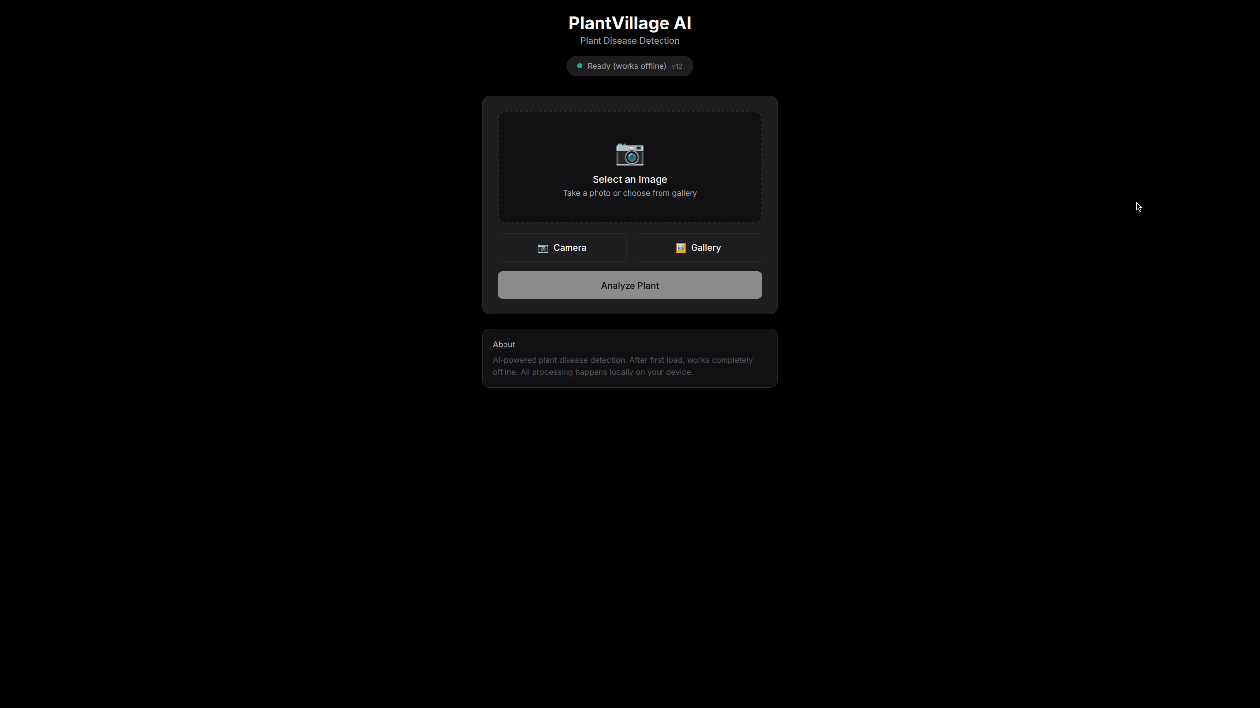
The PWA runs entirely offline via Service Worker. The first load caches the ~1.8MB ONNX model, and from that point it is airplane-mode ready. One critical detail: I had to write a custom bilinear resize in JavaScript that exactly matches PIL/Pillow's implementation to ensure consistent preprocessing between the training pipeline and browser inference. A 1-pixel difference in resize interpolation will silently destroy accuracy.
Benchmarks
Standardized benchmarks across hardware configurations. All tests: 100 iterations, 10 warmup, batch size 1, 128x128 input.
Burn (Rust) on CUDA
| Model Version | Mean (ms) | p50 (ms) | p99 (ms) | Throughput |
|---|---|---|---|---|
| Baseline | 0.41 | 0.31 | 0.93 | ~2,428 FPS |
| SSL | 0.42 | 0.25 | 1.09 | ~2,406 FPS |
Hardware Comparison
| Device | Latency | Throughput | Cost |
|---|---|---|---|
| Laptop (RTX 3060) | 0.42ms | ~2,406 FPS | €0 (BYOD) |
| Jetson Orin Nano | ~120ms | ~8 FPS | €350 |
| iPhone 12 (Tauri Mobile / Rust) | ~80ms | ~12 FPS | €0 (BYOD) |
| CPU Only | ~250ms | ~4 FPS | €0 |
The Jetson numbers were surprising. At €350 it was 8x slower than a phone the farmer already owns. That led to pivoting entirely to a BYOD (Bring Your Own Device) strategy. Every device hits the <200ms real-time target except bare CPU, which still comes in at 250ms.
Incremental Learning
A model that cannot learn new diseases post-deployment has an expiration date. I built an incremental learning system with four strategies, all implementing a generic Rust trait:
pub trait IncrementalLearner<B: Backend> {
    fn learn_incremental(
        &mut self,
        new_data: &[DataPoint],
        config: &IncrementalConfig,
    ) -> IncrementalResult;
}
Fine-tuning
Retrain on new data. Simple, but risks catastrophic forgetting of previously learned classes.
LwF (Learning without Forgetting)
Knowledge distillation from the old model. Preserves prior knowledge without storing training data.
EWC (Elastic Weight Consolidation)
Uses the Fisher information matrix to penalize changes to important weights. Memory-efficient and principled.
Rehearsal
Memory replay with herding, random, or distance-based sample selection from previous tasks.
This means a farmer could photograph a new disease variant, have an expert label a small batch, and the model updates itself on-device. No cloud round-trip, no redeployment.
Lessons Learned
- Burn is production-ready for inference. The API is clean, the multi-backend system works, and the community is responsive. Training ergonomics are still maturing compared to established frameworks.
- ONNX is the pragmatic bridge to the browser. Rather than fighting to compile Burn directly to WASM, exporting to ONNX and letting ONNX Runtime Web handle inference was the practical path. Ship what works.
- Dedicated edge hardware is often overkill. The Jetson costs €350 and was slower than the phone. Consumer devices are fast enough for most inference tasks at this model scale.
- Preprocessing parity is non-negotiable. A subtle difference in resize interpolation between training and inference silently destroys accuracy. Match your preprocessing pipeline exactly across all targets.
- Rust's compile times are real. Plan for 5+ minute release builds. Incremental debug builds are fast, but CI and release cycles feel the weight.
- Tauri v2 is well-suited for ML applications. Rust backend with a web frontend gives you native GPU access with modern UI tooling. The command/event system bridges both worlds cleanly.
Conclusion
What started as "can we run ML on a farm?" became a full exploration of Rust's ML ecosystem. The answer is yes, with caveats.
The semi-supervised pipeline turned 20% labeled data into results comparable to 60% labeled training. The Burn framework compiled the same model to desktop GPU, CPU fallback, and (via ONNX) the browser. Tauri v2 tied it together into a real application with a proper GUI.
Rust's ML ecosystem is still young compared to Python's, and there are rough edges. But for the specific problem of getting a trained model onto constrained devices that need to work offline, it delivered exactly what was needed. The entire project, from data loading to augmentation to training to inference, runs in one language. That simplicity has real engineering value.